NDArray; or N-Dimensional Array is the core data structure for most deep learning frameworks. It is a data structure that is able to hold a large amount of data in a single object, and it is highly optimized for matrix operations. In this post, we will discuss the basics of NDArray, how to create them, how to perform basic operations on them and how to use them to perform matrix operations.

Intruduction

There are two kinds of people, those with the curiosity to know what they are using, those who simply use. Le me, 28 March 2019.

There are many software packages and APIs for dealing with arrays. Among these is the famous numpy package. It is a wonderful peace of software that solved many data scientists problems through its amazing features and high performance speed (for a python library at least). In this post, I would like to introduce you to NDArrays and how they actually work, in python and the same goes for any other language (or most of them at least). In case you didn’t know, I love understanding the details of various libraries and tools especially those that goes around deep learning and scientific computing in general. So without further ado, let’s get started.

What is an ND-Array … ?

NDArray stands for N Dimensional Arrays. Simple right? I sure hoped it was until I started re-implementing it in C, for my Tensor library. For this tutorial however, we will be implementing NDArrays in python, just for the sake of simplicity. Our library will by no mean outperform numpy, but we will have some insights on how the latter works in details. Do note that numpy internally uses C/C++ APIs for higher performance and BLAS or Intel’sMKL (which I will talk about in a future post) for optimized matrix/vector operations.

NDArrays abstracts basic mathematical objects and even the complicated ones, such as vectors, matrixes, 3D matrixes (with depth) etc. You can think of those objects as tensors as well. For instance, wikipedia defines tensors as

A geometric object that maps in a multi-linear manner geometric vectors, scalars, and other tensors to a resulting tensor. Vectors and scalars which are often used in elementary physics and engineering applications, are considered as the simplest tensors. https://en.wikipedia.org/wiki/Tensor

Notes Before we start

Matrices are indexed in a row major order. If M is a matrix, M[0]`` refers to the first row, M[1] refers to the second row and so on. `M[i][j] Refers to the i-th row and j-th column.

Tensor vs NDArray

Now, you may be a bit confused about Tensors and NDArrays, what makes them different. Tensor is a rather common name used across mathematical and physical field, while NDArray refers to the technical implementation of tensors.

Tensor Representation & Memory

So, let’s imagine few mathematical objects such as a scalar, vector, matrix and a 3D matrix along with their representation. I might also include Some C pointers (might be also known as references objects in Java) here and there, because every language (e.g Python) uses C objects on its Virtual Machine, thus the same concept applies.

Scalar

Fig. 1: A Scalar Example

Now, a scalar can be simply represented as a single scalar variable in any language.

Vector

Fig. 2: Vector Representation

In C family, Vector is treated as a contiguous memory block. There is no padding between two consecutive elements of the same vector. Let’s assume here that x is an array of float. A single float takes about 32bits of memory, an array of size 1000 takes exactly 1000*32 bits. This is a huge advantage, as once you know the base array pointer index in memory (which is actually the variable you have declared) you can access any object in a O(1) time.

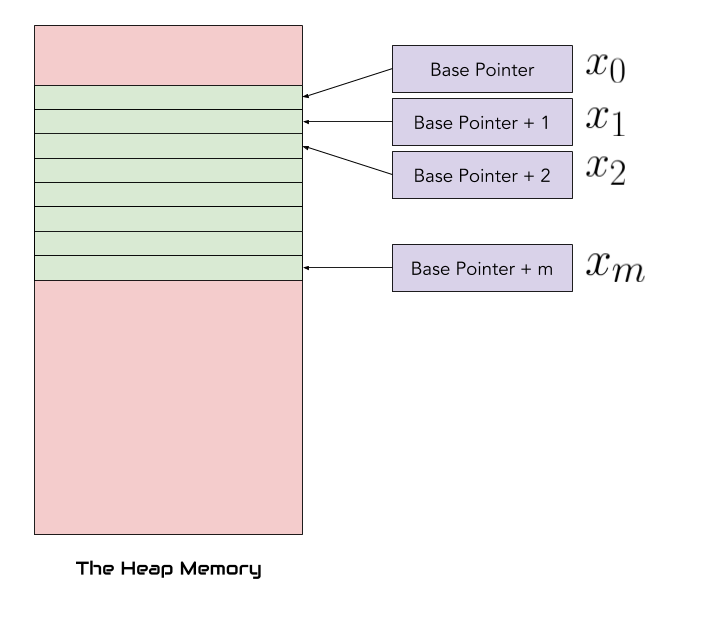Fig. 3: Vector, as stored in heap memory (RAM), where m = n-1 (n size of the vector)

Matrix

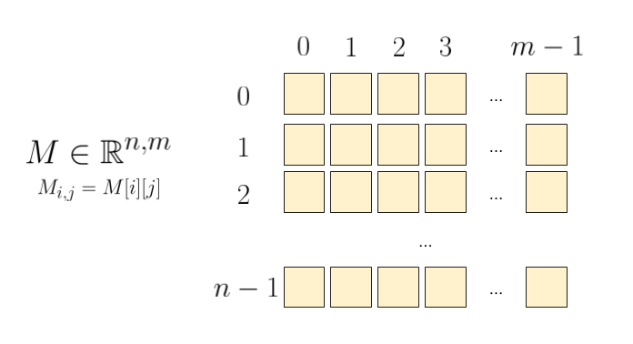Fig. 4: Matrix of n rows and m columns

Arrays are pretty simple. Let’s add one more dimension. We now have arrays of arrays! The easiest way to represent a matrix is to treat each row as single array, each element of this array points to another array! But first, let’s define a Matrix mathematically.

Now let’s talk about Matrix representation in memory. The EZ way is to create a table of rows and for each row allocate a new array, the pseudo code looks like this:

n = 5
m = 3

# create table
T = []

# create columns for each row
for i in range(n):
    T.append([0, 0, 0])

The previous python code will allocate memory in the following fashion: 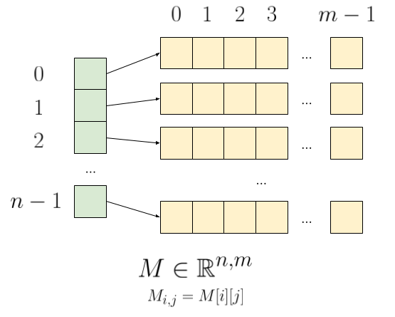Fig. 5: Each row of the matrix is actually an array (i.e pointer to another memory bloc)

While the rows of the matrix are contiguously allocated and each column is contiguously allocated on its own, the overall matrix is fragmented! There will be some random memory between each column of the matrix, as depicted in the figure 6. 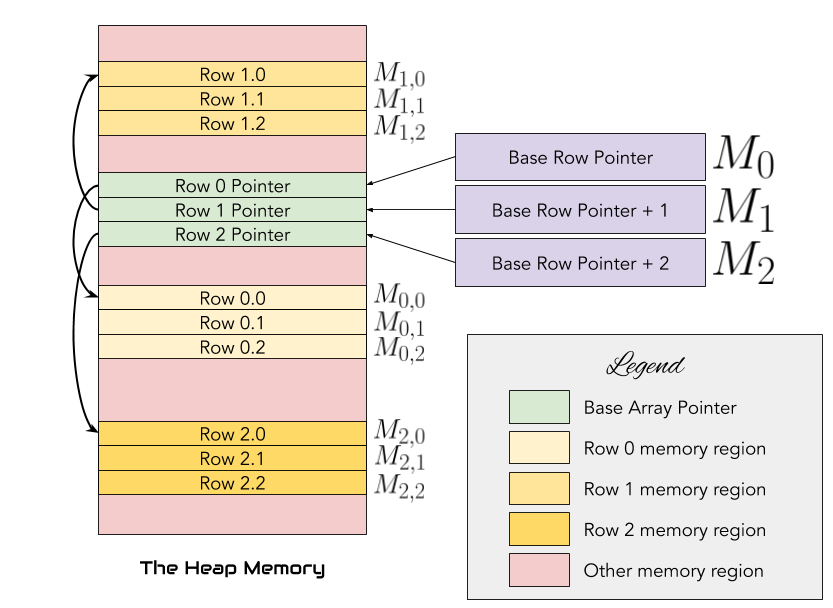Fig. 6: Memory allocation of arrays of arrays.

Allocating matrices in a such fashion is usually a bad choice since memory is fragmented and it disallows many optimizations, for instance, consider the case of passing a matrix to a GPU for some parallel processing, you would need to copy the data row by row which would make it harder. Thus, we, good ol’ people, prefer to use plain arrays. Additionally, in the previous example, we are allocating extra memories to hold the array value of each row.

Matrix as Plain Arrays (Matrix Flattening)

First of all, an NxM Matrix has a total size of … N*M. This will be the size of our array. What we need next is to come up with a formula, that maps each unique index (i, j) for the matrix, into a unique index k for the vector. Fortunately this is relatively easy, as we can simply use the following indexing technique: Eq. 1: 2D index to 1D Index mapping, M is a Matrix and V is a Vector.

Personally, when I knew about this formula, it was easier than I thought it would be. It is used especially when parallelizing code through threads or GPUs to copy the matrix in one operation. But now, let us visualize how a 2D Matrix is mapped into a single array in code and figures! 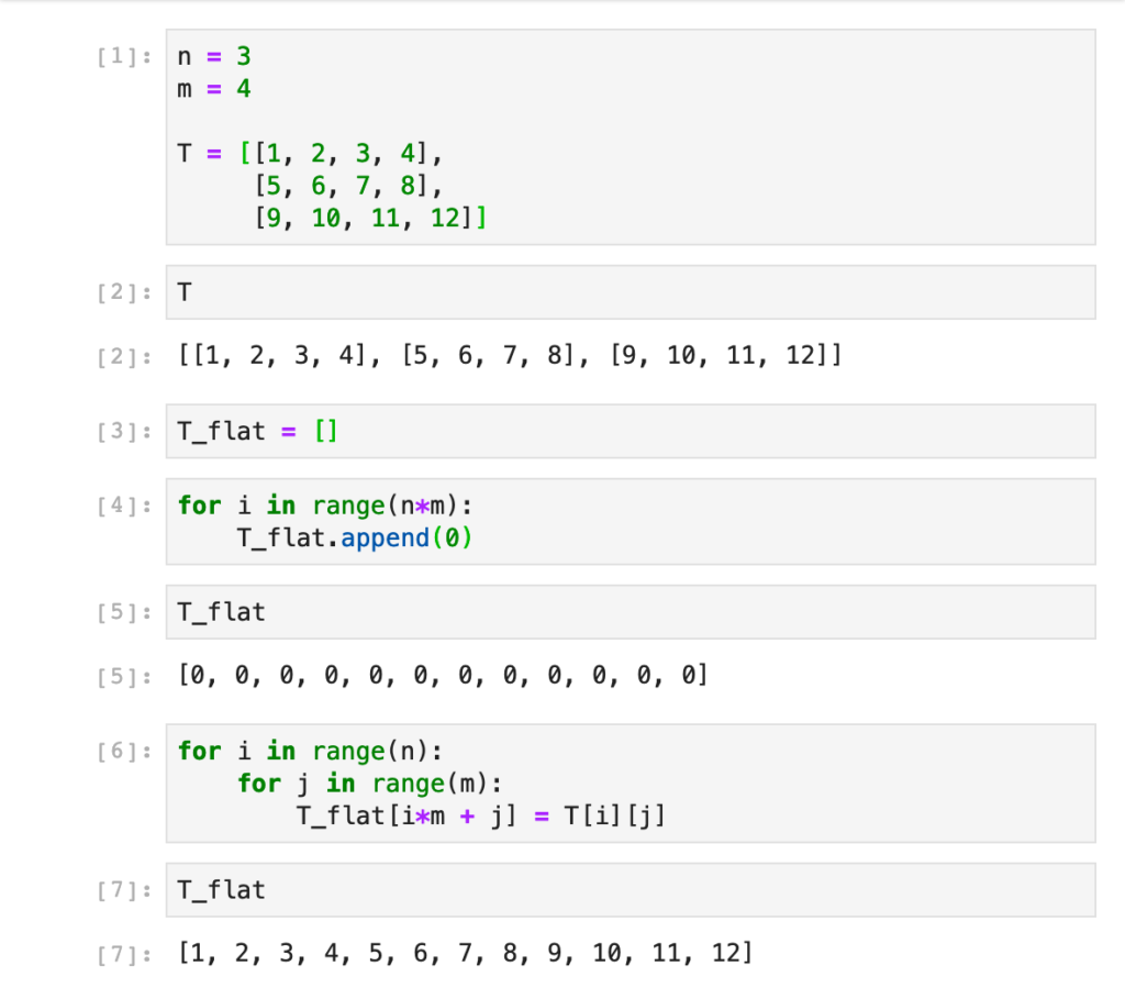Fig. 7: Matrix to array

As you can see, the vector is organized as sequence of matrix rows. Which raises another question, how do we go back from vector to matrix? I will give the answer right below, but do think about it for a second!

% Fig. 8: Cute cat to help you think (source: https://pixabay.com/photos/cat-sweet-kitty-animals-feline-323262/)

Array to Matrix (Reshape)

This one is easy enough. The array is ordered by rows. We have n rows. Each row contains n scalars (number of columns). Eq. 2: Mapping from 1D index k to 2D index (i, j), where i is the integer division betweenk and m, and j is the rest of division (modulo) between k and m (i.e % operator in C/C++). 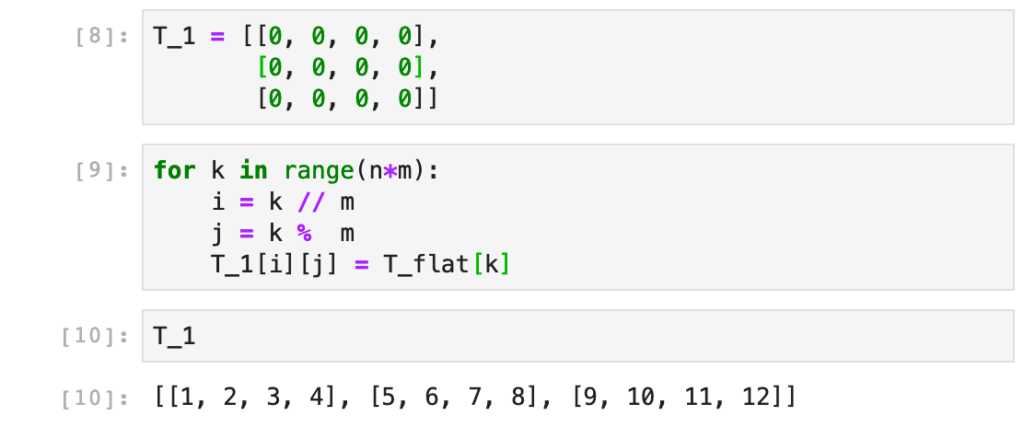Fig. 9: Array to matrix. Neat. Here is the notebook, if you insist.

Now that we know how to transform matrices to flat arrays and backwards, it is reasonable to use flat arrays for efficient memory allocation and access. In fact, numpy uses flat arrays internally. With smart indexing techniques, numpy can abstract all of this and support N-Dimensional arrays, that is higher order tensors. Before moving on, let’s review 3D Matrices and how to map them to flat arrays so we can up with a formula that can maps any Tensor to flat array.

3D Matrix

3D Matrix refers to stacked normal matrices. Stacked refers to another dimension, since matrices are two dimensional (rows and cols), adding another dimension (depth) will result in a 3D object. A very simple example of 3D Matrices are Images. Fig. 10: RGB Image. (source: https://pixabay.com/photos/animal-cat-close-up-eyes-feline-1834409/)

There many image extensions jpeg, png, tiff, etc. I will consider only png and jpeg to explain 3D Matrices. Both of these formats allows you to compress images with a quality/size tradeoff. But most interestingly, JPEG supports 3-channels images while PNG supports 4-channels images. 3 and 4 are the depth of an image. The most basic color space you probably know is RGB (Red, Green and Blue) where this tuple can be used to generate any possible color in the visible spectrum. 4-Channel images adds another channel to RGB, which is a for alpha. It is the transparency factor of a pixel. Transparency is usefull when editing picture or rendering them on a web page, where the background of the image is replaced with the color it has on its back, instead of filling it all with white. This tuple is RGBA.

The following notebook demonstrates how to split channels of RGB images using numpy.

Now, back to topic and straight to the point. Let’s make it formal and defined our new indexing strategy Eq. 3: 3D Index to 1D Index, through portals and black magic.

I suggest you try to implement that formula in python, same as I did for 2D arrays, hit me up if you have any problem. I, however, took a bigger challenge, which is to implement an NDArray Indexing to flat array.

Generalizing to NDArrays

Eq. 4: Generalizing Flattening indexes to m index spaces. (Do note that I have generated the equation my self after some deep research, and tested it for up to m = 4, if you find any inconsistencies please let me know)

Consider the case m=3, which is the previous example, try to evaluate the formula and you should get the same Eq. 3. And also, if m=2, you should get the same as Eq. 1 When we implement the formula above, we actually get a bit smart, we notice that each index i is multiplied by all the dimension of the shape starting from i+1 all the way to the end as is Figure 11.

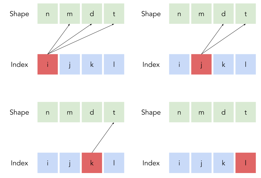Fig. 11: Index dependencies for a 4D space index, each index is multiplied with a set of dimension sizes which forms some pattern that we can code efficiently.

So, time for code, but first, let me explain the algorithm. First, both the shape of the Tensor and the indices are tuples of the same size (we are considering slices here). The last index has no dependencies over the size of each dimension, so it is the value of our 1D index. Then, we initialize an accumulator for dimension with 1, since it will multiplied by each the value of each dimension. Index i will be multiplied by the size of dimensions i+1, i+2 … i+m-1 (again, zero based indexing). We iterate through the shape array backwards, each time we add the result of that multiplication the our index. Here comes the code:

from functools import reduce

class NDArray:
    def __init__(self, values, shape):
        # check consistencies of the input
        val_len = reduce(lambda x, y: x*y, shape)
        assert len(values) == val_len, "Cannot create NDArray, given data of size {} and shape of total size {}".format(len(values), val_len)
        
        
        # value are standard python lists, must be flat
        self.values = values
        # shape is a tuple
        self.shape = shape
    
    def get(self, index):
        dim_counter = 1
        i = len(self.shape) - 1
        data_index = index[i]
        
        for i in reversed(range(1, len(self.shape))):
            # make sure the ith index is not larger than the size of the ith dimension
            assert index[i] < self.shape[i], "index {} with value {} is larger or equal the dimension {}".format(i, index[i], self.shape[i])
            
            dim_counter *= self.shape[i]
            data_index += index[i-1] * dim_counter
        
        return self.values[data_index]
   
X = NDArray([0, 1, 2, 3, 4, 5, 6, 7, 8, 9], (2, 5))
X.get((1, 4))
# returns 9.

There you have it! One easy thing we can do next is to reshape the array, which is done by simply updating the shape value of the class, just as long as the new shape matches the total size of the elements.

Notebook

Future Work

This post has been long for me to write but hopefully informative for you. While I will be writing on other things, I an considering going deeper into NDArray, more specifically, broadcasting. So stay tuned and let me know if you enjoyed this post and what you would like me to talk about next.

References

• Prof. Robert A. Dalrymple CUDA slides: http://www.ce.jhu.edu/dalrymple/classes/602/Class12.pdf